Multi-Task Learning, a Sentiment Analysis Example

Imagine at an autonomous driving company, you are tasked with building an object detection solution to identify pedestrians, vehicles, traffic lights, and stop signs in images. How will you tackle this problem?

One simple approach is to frame a multi-label classification problem, which can be solved by building 4 binary classifiers. In this case, each classifier will be in charge of identifying one of the aspects within our interest, such as traffic lights. However, building multiple independent models can be tedious especially if there are dozens of aspects you need to work on. Given the fact that we aim to solve multiple problems with the same nature of image classification, is it possible for us to develop an all-in-one solution to simultaneously address all the problems? This leads to the topic of this article, multi-task learning (MTL).

The general idea of MTL is to learn multiple tasks in parallel by allowing the lower-level features to be shared across the tasks. The training signals learned from one task can help improve the generalization of the other tasks. Let’s take a look at an example using MTL for aspect based sentiment analysis.

Problem Statement & Dataset

Aspect based sentiment analysis (ABSA) requires us to identify the polarity of text data with respect to multiple aspects relevant to the business use case. In ecommerce, extracting sentiment for different quality specs from user reviews allow us to generate product ratings by features such as appearance, battery life, and cost efficiency. With the feature-wise product ratings, customers can gain a comprehensive understanding on the pros and cons of the product, and therefore make better purchase decisions.

Amazon product review

In this article, we are going to use a restaurant review dataset, which is well studied in the ABSA related research. The dataset was taken from SemEval 2014, an international NLP research workshop. The training and test datasets contain 3041 and 800 restaurant reviews with annotations for 5 common aspects: service, food, anecdotes/miscellaneous, price, and ambience. A snippet of the raw data is given as follows.

<?xml version="1.0" encoding="UTF-8" standalone="yes"?>
<sentences>
    <sentence id="3121">
        <text>But the staff was so horrible to us.</text>
        <aspectTerms>
            <aspectTerm term="staff" polarity="negative" from="8" to="13"/>
        </aspectTerms>
        <aspectCategories>
            <aspectCategory category="service" polarity="negative"/>
        </aspectCategories>
    </sentence>
    <sentence id="2777">
        <text>To be completely fair, the only redeeming factor was the food, which was above average, but couldn't make up for all the other deficiencies of Teodora.</text>
        <aspectTerms>
            <aspectTerm term="food" polarity="positive" from="57" to="61"/>
        </aspectTerms>
        <aspectCategories>
            <aspectCategory category="food" polarity="positive"/>
            <aspectCategory category="anecdotes/miscellaneous" polarity="negative"/>
        </aspectCategories>
    </sentence>

The first review sentence carries a sentiment towards service, whereas the second review has sentiments for both food and anecdotes/miscellaneous. The raw data is in the .xml format. To make our life eaiser, we can parse the review sentences and sentiment labels into the standard table format using the xml.dom API from Python.

                                                text      food   service  ambience   price    misc
0                                  staff horrible us  negative    absent    absent  absent  absent
1                               bread top notch well  positive    absent    absent  absent  absent
2                say one fastest delivery times city    absent  positive    absent  absent  absent
3                    food always fresh hot ready eat  positive    absent    absent  absent  absent
4                         mention coffee outstanding  positive    absent    absent  absent  absent

Althought the sentiment labels were created for 5 aspects, it is not necessary for a review to have labels available for all the aspects. In fact, each review in the training data has labels for ~1.2 aspects on average. Here I impute the missing labels with “absent”. Our task is to make predictions for the sentiment of all 5 aspects. To tackle this multi-task problem, we are going to build a multi-head deep learning model. Let’s go!

Data Splitting

It can be observed that in the review data, there are multiple classes within each aspect. With pandas’ value_counts function, we can have a quick overview on the distribution of labels for different aspects. There are more than just positive and negative labels.

          service  food  anecdotes/miscellaneous  price  ambience
absent       2441  1806                     1911   2717      2607
positive      324   867                      544    179       263
negative      218   209                      199    115        98
conflict       35    66                       30     17        47
neutral        20    90                      354     10        23

Interestingly, in addition to the typical positive, negative and neutral labels, we also see some reviews with a “conflict” label. Conflict indicates that both positive and negative sentiment were detected from a review. Here’s one example of such reviews.

It took half an hour to get our check, which was perfect since we could sit, have drinks and talk!

To split the given training data for model training and validation, we’d like to maintain the proportion of different classes for all 5 aspects as much as possible. This can be achieved with the IterativeStratification module from the skmultilearn library. The idea is to consider the combination of labels from different aspects, and assign the examples based on the predefined training/validation split ratio. I used a train_size of 0.8 in practice. The following function was used to perform the stratified split of the data.

from skmultilearn.model_selection import IterativeStratification


def iterative_train_test_split(
    self, X: np.array, y: np.array
) -> Tuple[np.array, np.array]:
    """Custom iterative train test split which maintains the
    distribution of labels in the training and test sets
    Parameters
    ----------
    X : np.array
        features array
    y : np.array
        labels array
    Returns
    -------
    Tuple[np.array, np.array]
        indices of training and test examples
    """
    stratifier = IterativeStratification(
        n_splits=2,
        order=1,
        sample_distribution_per_fold=[
            1.0 - self.train_size,
            self.train_size,
        ],
    )
    train_indices, test_indices = next(stratifier.split(X, y))

    return train_indices, test_indices

Dataset Creation

To create the datasets for training our neural network. I first define a vectorizer class to tokenize the review words and convert them into pre-trained word vectors with a medium-sized English model provided by Spacy. This model can be replaced with a transfermer based model, which can potentially improve the accuracy of classification. Alternatively, we can train the embedding layer within the neural network. For the POC purpose, the Spacy model I chose is sufficient. It will help us quickly finish training the model.

Note that the Spacy model needs to be downloaded before being used.

import en_core_web_md


class ABSAVectorizer:
    def __init__(self):
        """Convert review sentences to pre-trained word vectors"""
        self.model = en_core_web_md.load()

    def vectorize(self, words):
        """
        Given a sentence, tokenize it and returns a pre-trained word vector
        for each token.
        """

        sentence_vector = []
        # Split on words
        for _, word in enumerate(words.split()):
            # Tokenize the words using spacy
            spacy_doc = self.model.make_doc(word)
            word_vector = [token.vector for token in spacy_doc]
            sentence_vector += word_vector

        return

Then we can create the dataset class as follows. Since we need to make predictions for 5 aspects, the sentiment labels need to be fed as a vector for each review.

from torch.utils.data import Dataset


class ABSADataset(Dataset):
    """Creates an pytorch dataset to consume our pre-loaded text data
    Reference: https://pytorch.org/tutorials/beginner/basics/data_tutorial.html
    """

    def __init__(self, data, vectorizer):
        self.dataset = data
        self.vectorizer = vectorizer

    def __len__(self):
        return len(self.dataset)

    def __getitem__(self, idx):
        (labels, sentence) = self.dataset[idx]
        sentence_vector = self.vectorizer.vectorize(sentence)
        return {
            "vectors": sentence_vector,
            "labels": labels,
            "sentence": sentence,  # for debugging only
        }

Model Training

Now it’s time to build our neural network. How can we enable our network to handle multiple tasks at the same time? The trick is to create multiple “heads” so that each “head” can undertake a specific task. Since all tasks need to be tackled based on the same set of features created out of the reviews, we need to declare a “backbone” to connect the source features with the different “heads”. That’s how we arrive at the following network architecture.

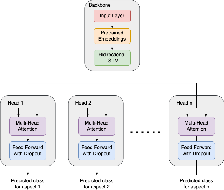
The Sequential API provided by Pytorch can help us declare the “heads” with a loop. Within each “head”, a vanilla attention layer is introduced. The implementation of the attention layer can be found here. Based on my experiment, adding the attention layer improved the model accuracy by ~10%.

from typing import List

import torch
from omegaconf import DictConfig

from attention import MultiHeadAttention


class MultiTaskClassificationModel(torch.nn.Module):
    def __init__(
        self,
        aspects: List[str],
        num_classes: int,
        hyparams: DictConfig,
    ):
        super().__init__()
        self.aspects = aspects
        self.backbone = torch.nn.LSTM(
            input_size=hyparams.word_vec_dim,
            hidden_size=hyparams.hidden_dim,
            num_layers=hyparams.num_layers,
            batch_first=True,
            bidirectional=True,
        )  # Output dimension = (batch_size, seq_length, num_directions * hidden_dim)

        # Define task specific layers
        num_directions = 2
        self.heads = torch.nn.ModuleList([])
        for aspect in aspects:
            module_name = f"h_{aspect}"
            module = torch.nn.Sequential(
                MultiHeadAttention(
                    embed_dim=hyparams.hidden_dim * num_directions,
                    num_heads=hyparams.num_heads,
                ),
                torch.nn.Linear(
                    hyparams.hidden_dim * num_directions, int(hyparams.hidden_dim / 2)
                ),
                torch.nn.Dropout(hyparams.dropout),
                torch.nn.Linear(int(hyparams.hidden_dim / 2), num_classes),
            )
            setattr(self, module_name, module)

    def forward(self, batch, batch_len):
        """Projection from word_vec_dim to n_classes
        Batch in is shape (batch_size, max_seq_len, word_vector_dim)
        Batch out is shape (batch, num_classes)
        """

        # This deals with variable length sentences. Sorted works faster.
        packed_input = torch.nn.utils.rnn.pack_padded_sequence(
            batch, batch_len, batch_first=True, enforce_sorted=True
        )
        lstm_output, (h, c) = self.backbone(packed_input)
        output_unpacked, _ = torch.nn.utils.rnn.pad_packed_sequence(
            lstm_output, batch_first=True
        )
        hs = [getattr(self, f"h_{aspect}")(output_unpacked) for aspect in self.aspects]
        return torch.cat(hs, axis=1)

The total loss of the multi-task network can be calculated by aggregating the cross entropy losses from all the heads. We can skip calculating the loss for the aspects with no label, since we are not interested in making prediction for them. This is also aligned with the evaluation methodology specified by SemEval-2014. The accuracy is also computed with the “absent” aspects skipped.

from typing import Dict, List

import numpy as np
import torch
import pytorch_lightning as pl
import torch.nn.functional as F
import torchmetrics


class ABSAClassifier(pl.LightningModule):
    def __init__(
        self,
        model,
        aspects: List[str],
        label_encoder: Dict[str, int],
        learning_rate: float,
        class_weights: List[float],
    ):
        super().__init__()
        self.model = model
        self.aspects = aspects
        self.label_encoder = label_encoder
        self.num_aspects = len(self.aspects)
        self.learning_rate = learning_rate
        self.class_weights = torch.tensor(class_weights)
        self.acc = torchmetrics.Accuracy()

    def forward(self, x, x_len):
        return self.model(x, x_len)

    def _calculate_loss(self, batch, mode="train"):
        # Fetch data and transform labels to one-hot vectors
        x = batch["vectors"]
        x_len = batch["vectors_length"]
        y = batch["labels"]  # One-hot encoding is not required

        # Perform prediction and calculate loss and F1 score
        y_hat = self(x, x_len)
        agg_loss = 0
        total_examples = 0
        correct_examples = 0
        for idx, _ in enumerate(self.aspects):
            prob_start_idx = self.num_aspects * idx
            prob_end_idx = self.num_aspects * (idx + 1)

            # Skip data points with the "absent" label
            valid_label_ids = np.where(y[:, idx] != self.label_encoder["absent"])[0]
            if len(valid_label_ids) > 0:
                loss = F.cross_entropy(
                    y_hat[valid_label_ids, prob_start_idx:prob_end_idx],
                    y[valid_label_ids, idx],
                    reduction="mean",
                    weight=self.class_weights,
                )
                agg_loss += loss

            predictions = torch.argmax(
                y_hat[valid_label_ids, prob_start_idx:prob_end_idx], dim=1
            )
            correct_examples += torch.sum(predictions == y[valid_label_ids, idx])
            total_examples += len(valid_label_ids)
            acc = correct_examples / total_examples

        # Logging
        self.log_dict(
            {
                f"{mode}_loss": agg_loss,
                f"{mode}_acc": acc,
            },
            prog_bar=True,
        )
        return agg_loss

Across all 5 aspects, a majority of the review data fall under the “positive” and “negative” categories. To tackle the class imbalance, we can assign higher weights for the examples under “conflict” and “negative” categories. This technique can lead to a slight increase of the accuracy.

Results and Conclusion

After training the multi-task network for 3 epochs, we evaluate its performance with the unseen test dataset. An overall accuracy of 0.7434 can be achieved. This is ~10% higher than the baseline test accuracy obtained with the naive majority class classifier. Let’s also look at the breakdown of accuracy for different aspects.

Aspect	Majority class accuracy	MTL accuracy
food	0.7225	0.7823
service	0.5872	0.8430
price	0.6145	0.7590
ambience	0.6441	0.7542
anecdotes/miscellaneous	0.5427	0.5897
overall	0.6410	0.7434

Our multi-task network model outperforms the baseline in all 5 aspects, although the accuracy for anecdotes/miscellaneous is below 0.6. It is potentially due to the high proportion of the neutral examples from this aspect.

One future work for further validating the MTL approach is to train 5 independent multi-class classification models for individual aspects, and compare the accuracy. It’s highly likely that we will end up with a poor accuracy for the price and ambience aspects due to their small volume of data. In this problem the superior performance of MTL is brought by the effect of data enrichment across different tasks. MTL typically works well under the following conditions.

There are multiple highly similar problems to solve.
There is sufficient amount of data relevant for solving all the problems.

Hope this example can give you a basic understanding of multi-task learning, and how it can be applied to tackle a practical problem. The full code for this blog can be found on GitHub.

References

Written on October 23, 2022