
Crack Site Selection Puzzle by Geospatial Analysis (Part 2)
Photo by author
In the first blog of this series, we developed an idea aiming to address the site selection problem from the perspective of the demand and supply. We completed the analysis of the demand side and simulated the distribution of the customers in the target city, Penang. Although the case study is conducted in the scenario of the grocery industry, the same solution can be applied to real estate, e-commerce, and education sectors as well. In this blog, we are going to tackle the supply side and look into the imbalance between the demand and supply across the city. Bear in mind that our client is a supermarket chain and its potential customers are the entire population of the city.
The supply analysis consists of the following sections.
- Competitor discovery: to find the locations of the existing supermarkets and grocery stores.
- Distance estimation: to estimate the distance between the competitor outlets and the different locations around the city.
- Customer density estimation: to estimate the average number of customers served by one supermarket or grocery store at different locations of the city.
Competitor Discovery
The information about existing grocery providers can be obtained using the Google Places API. It provides a variety of information about different types of places of interest, including their outlet name, geographical location, opening hours, and even visitor ratings etc. Here we expect the information provided by the API is up to date. However, it is not guaranteed that the API can detect all the places which fulfil the search criteria, especially for the less developed regions. For the purpose of this study, this is the best accessible data source we can rely on.
The Places API works with an API key and is usually queried with 3 parameters: the type of amenity, a center location, and a radius. Recap in the first series, we split the entire city area into thousands of 1km x 1km grids. In order to collect all the existing grocery providers available via the API, we take the geo-coordinates of the grid centers, and search for the supermarkets and grocery stores within 2 km’s distance. To make the blog more concise and less heavy with code, I’m going to omit the preparatory steps of the input data and the config parameters, and only highlight how the Places API is queried. The following code extracts the supermarkets within 2 km’s distance from Orchard Road, Singapore.
import googlemaps


API_KEY = "YOUR_API_KEY"
gmaps = googlemaps.Client(key=API_KEY)
res = gmaps.places(
    "supermarket",
    location="1.304833,103.831833",  # Orchard Road, Singapore
    radius=2000
)

if res["status"] == 'OK' and len(res["results"]) > 0:
    for result in res["results"]:
        print(result)
else:
    print("No place is found")
The query results are returned as a list of Python dictionaries. One of them looks as follows. In this study, we only use the geolocation information of the existing supermarkets.
{
   "business_status":"OPERATIONAL",
   "formatted_address":"491 River Valley Rd, #01-14, Singapore 248371",
   "geometry":{
      "location":{
         "lat":1.2929051,
         "lng":103.8270208
      },
      "viewport":{
         "northeast":{
            "lat":1.294498079892722,
            "lng":103.8284264298927
         },
         "southwest":{
            "lat":1.291798420107278,
            "lng":103.8257267701073
         }
      }
   },
   "icon":"https://maps.gstatic.com/mapfiles/place_api/icons/shopping-71.png",
   "id":"fda0ec60faa787f2bf992132e66c80f29daa5964",
   "name":"FairPrice Finest Valley Point",
   "opening_hours":{
      "open_now":False
   },
   "photos":[
      {
         "height":2048,
         "html_attributions":[
            "<a href=\"https://maps.google.com/maps/contrib/111973208857299784904\">Anusha Lalwani</a>"
         ],
         "photo_reference":"CmRaAAAAQ6An4L-A5PbgDFkpZVllEGuB4Ayw0hdrZ9coCBaF6esLM2B7RVnJCvf0DPeZrlcbZ3KVFUz9cciPtArUAZ6tof_lJHzJHqKzcEFyRGJurK_Drld0GUec9sCWm25bXURVEhD6GZqf6j_Kb5IOTtQ1ogslGhQas22jzBT2rJ0jkj9zUhDvCLYj_w",
         "width":1536
      }
   ],
   "place_id":"ChIJTyWXW4EZ2jERNKBCOx_-4LA",
   "plus_code":{
      "compound_code":"7RVG+5R Singapore",
      "global_code":"6PH57RVG+5R"
   },
   "rating":4,
   "reference":"ChIJTyWXW4EZ2jERNKBCOx_-4LA",
   "types":[
      "grocery_or_supermarket",
      "food",
      "point_of_interest",
      "store",
      "establishment"
   ],
   "user_ratings_total":112
}
The supermarkets and grocery stores are collected from all the grids and plotted on the QGIS map after removing the duplicates, as shown in the following graph. It can be observed that the distribution of the existing grocery providers (the white dots) is approximately aligned with the customer distribution.
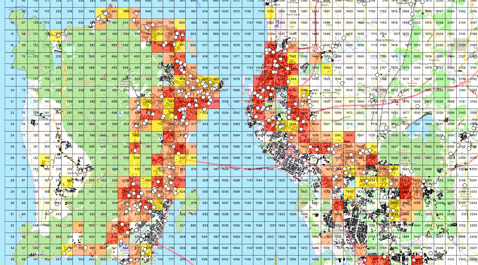
Partial view of the existing supermarkets and grocery stores across Penang city
Distance Estimation
Allow me to ask you a question. How long would you like to spend on travelling for grocery shopping?
People living in different cities could have different answers. My answer to this question is 15 min’s walking distance. Walking to the grocery store can be taken as a regular physical exercise during a lockdown. In this study, we are expecting a longer threshold of travelling time due to the relatively small population density of Penang. According to the advice given by a friend from Malaysia, we assume a threshold of 10 min’s driving distance. It is the most important parameter used in this analysis and can be adjusted easily if the solution is deployed as a dashboard application later on. Please note that in consulting projects, such parameters need to be obtained via rigorous market research.
This travelling distance question is important here because, given the threshold of the travelling time, we can estimate the number of customers each grocery store can reach out to, which is known as catchment analysis. To facilitate this analysis, we extract the estimated driving time between each pair of grid and existing grocery store via Google Distance Matrix API. The following code extracts the driving time from Orchard Road to Marina Bay Sands, Singapore.
import googlemaps


API_KEY = "YOUR_API_KEY"
gmaps = googlemaps.Client(key=API_KEY)
ORCHARD_ROAD = (1.304833, 103.831833)
MARINA_BAY_SANDS = (1.282302, 103.858528)
res = gmaps.distance_matrix(
    ORCHARD_ROAD,
    MARINA_BAY_SANDS,
    mode='driving'
)

print(res)
The result indicates that the driving time from the origin to the destination address is 13 min.
{
   "destination_addresses":[
      "10 Bayfront Ave, Singapore 018956"
   ],
   "origin_addresses":[
      "2 Orchard Turn, Singapore 238801"
   ],
   "rows":[
      {
         "elements":[
            {
               "distance":{
                  "text":"5.2 km",
                  "value":5194
               },
               "duration":{
                  "text":"13 mins",
                  "value":761
               },
               "status":"OK"
            }
         ]
      }
   ],
   "status":"OK"
}
Customer Density Estimation
Let’s summarise the key information we have obtained at grid level.
- Population, or number of customers for each grid.
- Number of grocery stores and supermarkets which serve the customers living in each grid.
Now we take a quick look at the distribution of the number of customers and the grocery stores across the grids. The grids with no population are ignored in the following histograms.
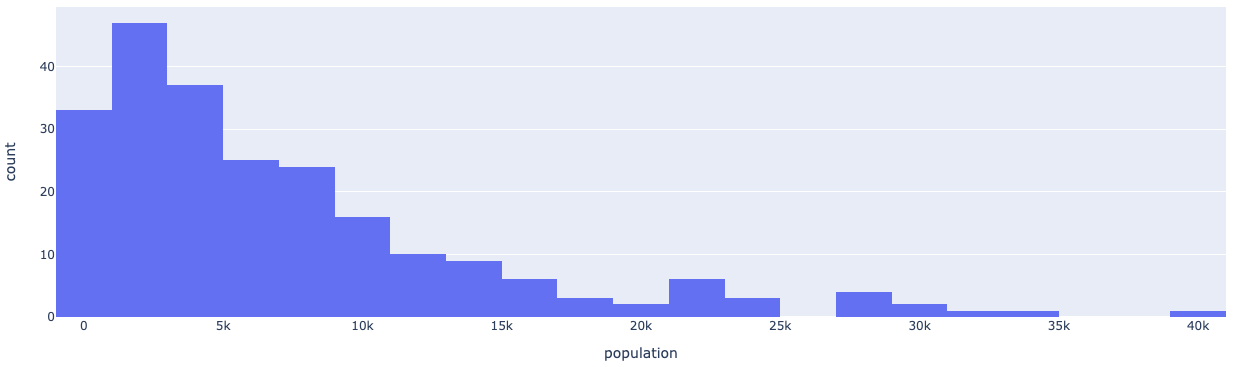
Distribution of the grid-wise number of customers
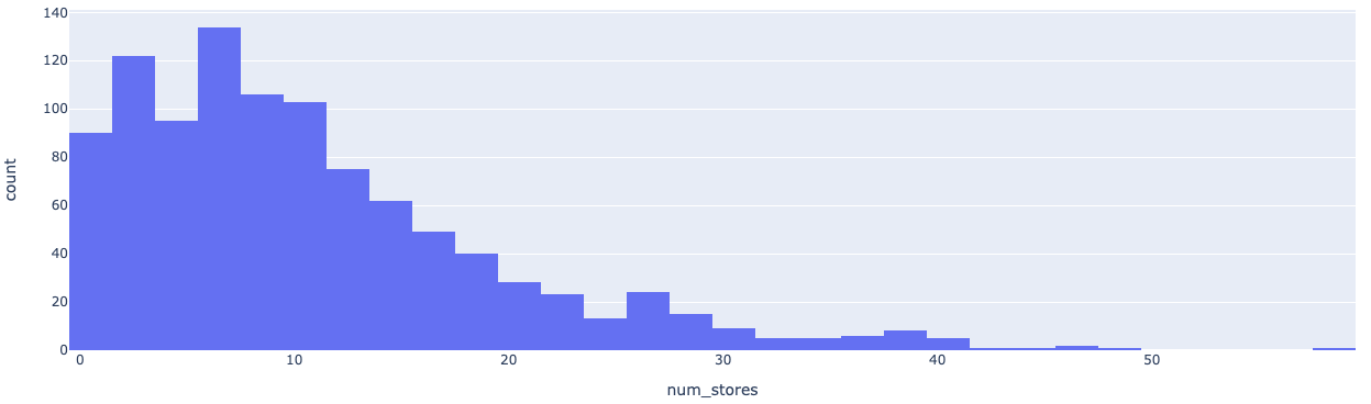
Distribution of the grid-wise number of outlets
Both the number of customers and grocery stores look reasonable. From here, we are going to calculate a customer density index for each grid to evaluate the imbalance of the demand and supply across the city. Conceptually, it is equivalent to the demand to supply ratio (DSR).
customer density = Number of customers / Number of grocery stores and supermarkets serving the customers in the grid
We are going to recommend locations of the new supermarkets based on the customer density value. In general, high customer density indicates a good location for the new outlets. Therefore, our client can use it as a reference for site selection.
The distribution of customer density across Penang can be visualized in the following heatmap. The regions with high DSR are highlighted in dark blue.
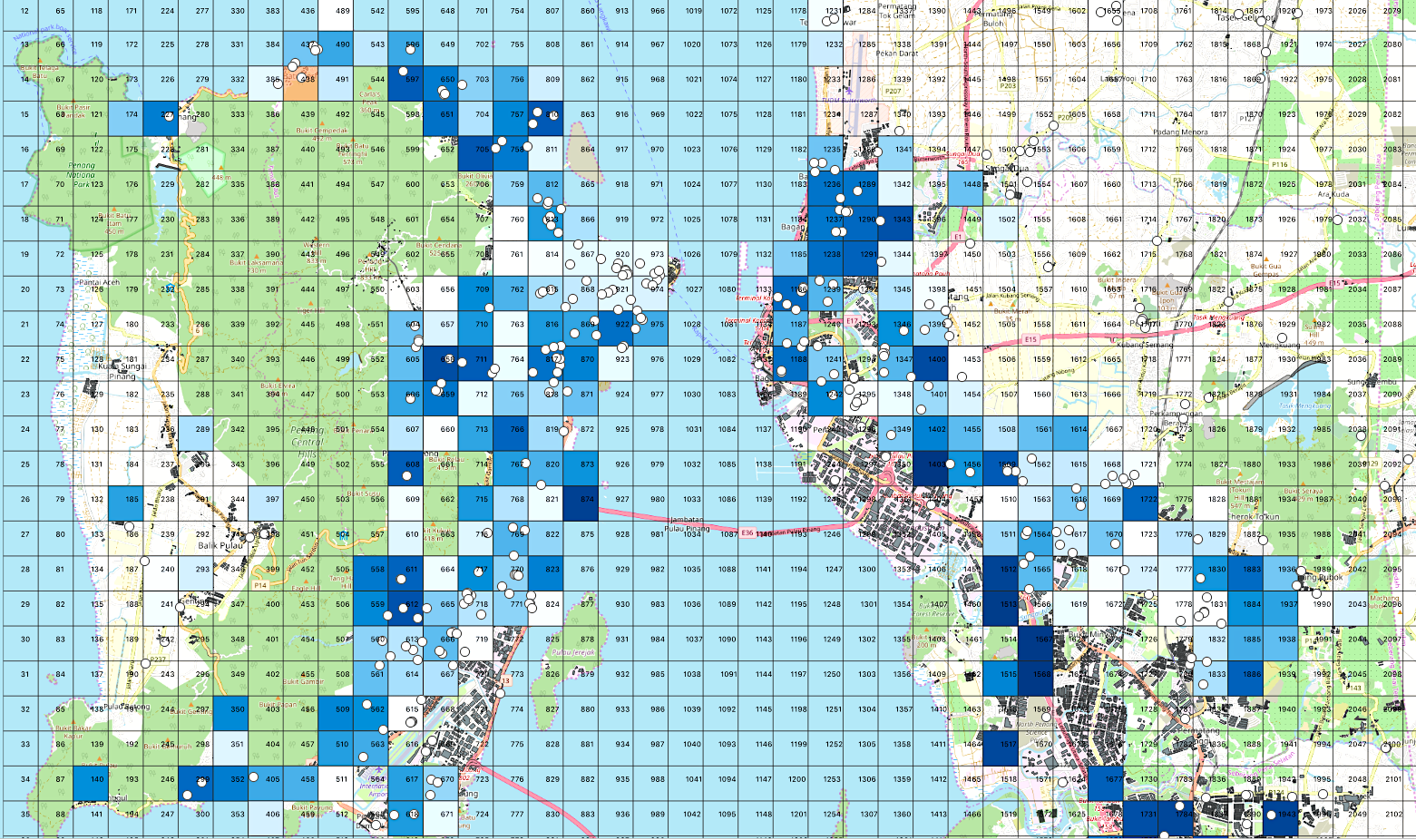
Distribution of customer density across Penang city
Final Words
This concludes the series of the site selection case study. You might have noticed that the capacity of the supermarkets is not considered when estimating customer density. In other words, the capacity of all the existing stores is treated the same in this study, which is not accurate in reality. One possible solution to this issue is to match the existing stores with their corresponding shapes from the OpenStreetMap (OSM) data. Floor area can be calculated with the coordinates and used to estimate the capacity of the stores.
In addition, please plan your queries of Google API before execution. Do an estimation of the number of queries and the total cost.
The scripts and notebooks used in this study are available on GitHub. Thanks for the read.