Site selection is a popular topic in the consulting industry. In this blog, I am introducing a novel solution backed by open source OpenStreetMap dataset and QGIS. Hope this case study can bring some fresh ideas to the analysts and consultants who work on the site selection related projects.

Problem Statement

Suppose we have a client, who is a supermarket chain. They plan to build their retail stores in a new city, say Penang, Malaysia. They need to decide how many outlets to build as well as where they should locate them in order to maximise the profits. It will become a complicated problem if we attempt to develop the solution from the perspective of predictive modelling. Profit seems to be an appropriate target variable to predict. However, it would take tremendous efforts to determine the features to use and compile the feature set.

The strategy I propose can be summarised with one sentence: “find out the locations with higher customer density and fewer competitors”. With this idea in mind, the problem can be approached with the following 3 steps.

1. Simulate the geographical distribution of the customers over the entire city.
2. Acquire the geographical locations of the potential competitors in the city, including any other supermarket chains, and grocery stores.
3. Propose locations of outlets according to the gap between the supply and demand in different areas.

This blog will focus on the first part: simulation of customer distribution.

• Input data: OpenStreetMap shape file of the buildings in Penang city, estimated Penang population distributed by districts.
• Tools in use: Python 3, QGIS (Quantum Geographic Information System) 3.4

Data Sources

Let’s first take a look at the data we will be working on. OpenStreetMap (OSM) is a collaborative project, aiming to create an open source editable map of the world. The dataset contains the shape files of various types of infrastructure such as buildings, roads, railways in the target region. The dataset gets updated every few hours. In order to obtain the OSM dataset of Penang, I downloaded the package of shape files for Malaysia, Singapore, and Brunei from the OSM website. There are a few Python libraries that can be used to process the shape files with the .shp suffix: Fiona, PyShp, Shapely, GeoPandas, etc. In this work, PyShp is used to read the shapefile into a dataframe.

import pandas as pd
import shapefile as shp


def read_shapefile(sf):
    """
    Read a shapefile into a Pandas dataframe with a 'coords'
    column holding the geometry information. This uses the pyshp
    package
    """
    fields = [x[0] for x in sf.fields][1:]
    records = [list(i) for i in sf.records()]
    shps = [s.points for s in sf.shapes()]
    df = pd.DataFrame(columns=fields, data=records)
    df = df.assign(coords=shps)

    return df


shp_path = 'raw/gis_osm_buildings_a_free_1.shp'
sf = shp.Reader(shp_path)
shp_df = read_shapefile(sf)

shp_df.head()

One interesting feature I would like to highlight is the coords, which gives the latitude and longitude of the vertices of the buildings in clockwise order. It can be used to estimate the specific location of the buildings as well as their floor area.

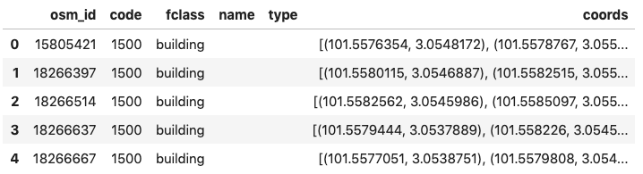
Shape file read as a pandas dataframe

The other data in use is the estimated Penang population distributed by districts, provided by Penang Institute. The latest data available by writing this article is from the Q4 2019 report, as shown in the following table.

Geographically Penang city is separated into Penang Island and Seberang Perai by the Penang Strait. The 5 districts of Penang can be visualised in the following map, quoted from Wikimedia Commons.

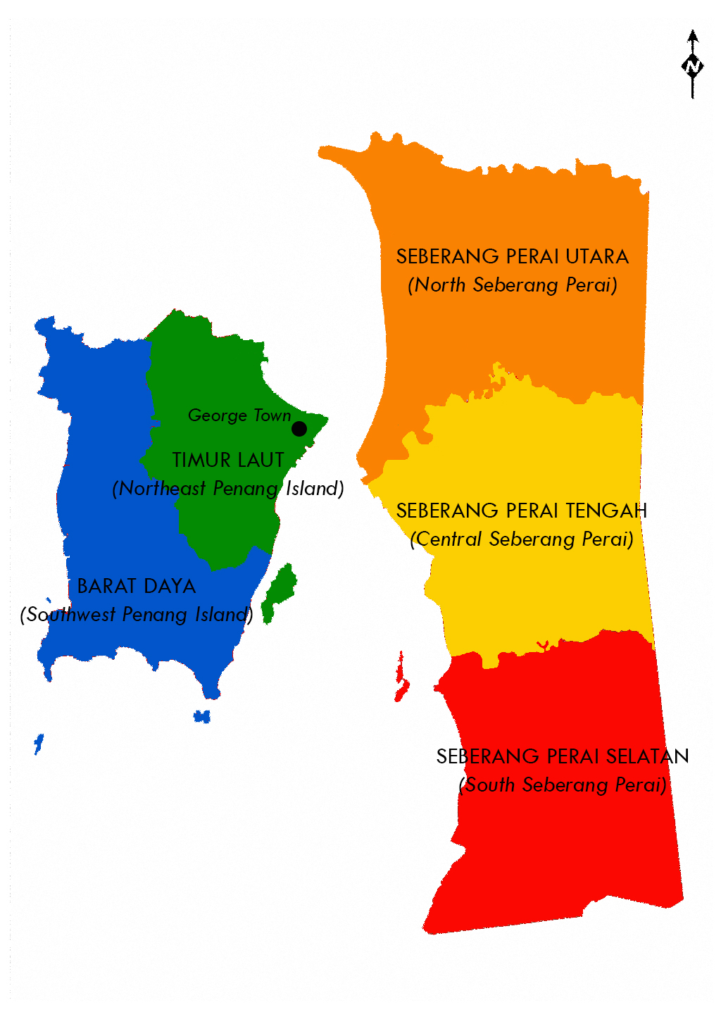
Districts of Penang

Simulation Approach and Assumptions

Here we have an overview of the methodology before we dive into the implementation. The customer distribution can be simulated in the following steps.

1. Estimate the centric geocode and floor area of all the residential buildings (Python).
2. Split Penang city into 1km x 1km grids and label which district they belong to respectively (QGIS).
3. Allocate the residential buildings to the grids according to the buildings’ centric geocode and calculate the gridwise floor area in total (Python).
4. Allocate the district population to grids based on their floor area (Python).

The solution makes sense with the following assumptions.

• The target customers of the supermarket outlets are the entire population of Penang.
• All the residential buildings can be classified into 2 types: apartments and bungalows.
• For each district, the residential density of the apartments is uniform. To be more specific, the residential density refers to the population per floor area.
• The residential density of bungalows is uniform over the city: 5 ppl / 100 m².

The third assumption indicates that all the apartments share a same number of floors. It is introduced to simplify the problem since the building height information is missing in the OSM dataset.

Implementation Walkthrough

Floor area calculation

After the shape file is read in as a dataframe, we need to select the entries of the residential buildings of Penang. This can be achieved by filtering the dataframe by the building type and the centric geocode of the buildings. The centric geocode is calculated by taking the average of the latitude and longitude of all the vertices of a building. The boundaries of Penang city is declared with the following ranges of geocode.

• latitude: 5.1175 – 5.5929
• longitude: 100.1691 – 100.5569

def get_center(coords):
    """Calculate the averge latitude and longitude of the vertices of a building
    """
    num_points = len(coords) - 1
    sum_lng = 0
    sum_lat = 0
    for i in range(num_points):
        point = coords[i]
        sum_lng += point[0]
        sum_lat += point[1]
    return (sum_lng / num_points, sum_lat / num_points)


def is_penang(geocode):
    """Check whether a building is within Penang based on its geocode
    """
    lat, lng = geocode[1], geocode[0]
    if lat > 5.1175 and lat < 5.5929 and lng > 100.1691 and lng < 100.5569:
        return True
    else:
        return False


# Select residential buildings
residential_types = [
    "condominium", "apartment", "apartments",
    "dormitory", "EiS_Residences", "residential",
    "bungalow", "detached", "mix_used"
]
residential_df = shp_df.loc[shp_df["type"].isin(residential_types)]
residential_df = residential_df.set_index("osm_id")
residential_df["center"] = residential_df["coords"].apply(
    lambda coords: get_center(coords)
)

# Boundary of Penang State, obtained from OSM
# lat: 5.1175 - 5.5929; lng: 100.1691 - 100.5569
residential_df["is_penang"] = residential_df["center"].apply(
    lambda geocode: is_penang(geocode)
)
penang_df = residential_df.loc[residential_df["is_penang"] == True]
penang_df.head()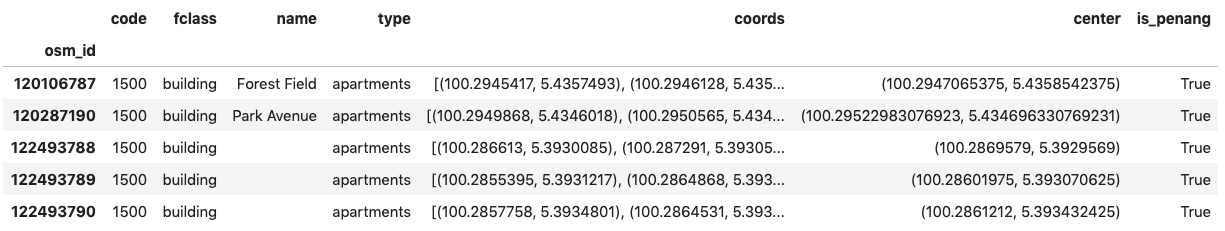

Dataframe of Penang residential buildings

The floor area of buildings can be estimated based on the geocode of the buildings’ vertices. Mapbox provides an API to calculate the area of a geojson polygon or multipolygon, which can be applied here.

import numpy as np
from area import area


def get_center(coords):
    num_points = len(coords) - 1
    sum_lng = 0
    sum_lat = 0
    for i in range(num_points):
        point = coords[i]
        sum_lng += point[0]
        sum_lat += point[1]
    return (sum_lng / num_points, sum_lat / num_points)


penang_df["area"] = penang_df["coords"].apply(
    lambda coords: calc_floor_area(coords)
)
penang_df["center_lng"] = penang_df["center"].apply(lambda geocode: geocode[0])
penang_df["center_lat"] = penang_df["center"].apply(lambda geocode: geocode[1])
penang_df["area"] = penang_df["coords"].apply(
    lambda coords: calc_floor_area(coords)
)
penang_df["id"] = np.arange(len(penang_df))
penang_df = penang_df.reset_index()
penang_df = penang_df.drop(
    ["osm_id", "code", "fclass", "is_penang", "center", "coords"],
    axis=1
)
penang_df = penang_df.set_index('id')
penang_df.to_csv("data/penang_residential_buildings.csv", index=True)

A snapshot of the exported data can be viewed below.

Discretisation of city using grids

The ultimate goal of the project is to propose locations of supermarket outlets in the city. Therefore, we are going to create grids and analyse the demand and supply with respect to the individual grids. The locations of outlets will be proposed in the form of grids. QGIS is an open-source desktop geographic information system application. It is used for this purpose since it provides various map manipulation and visualisation functions. Import the OSM shape file to QGIS, and create the grids using the Create Grid function.

Click Vector -> Research Tools -> Create Grid in sequence. The dialog box for grid creation looks as follows.

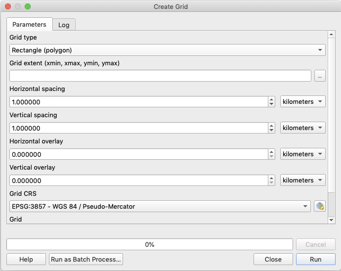
Create Grid function of QGIS

The Grid extent in the above dialog box is used to define the area covered by the grids. We can take the “Use Canvas Extent” option to manually drag-select a rectangular area which covers Penang. The generated grid layer is shown as follows.

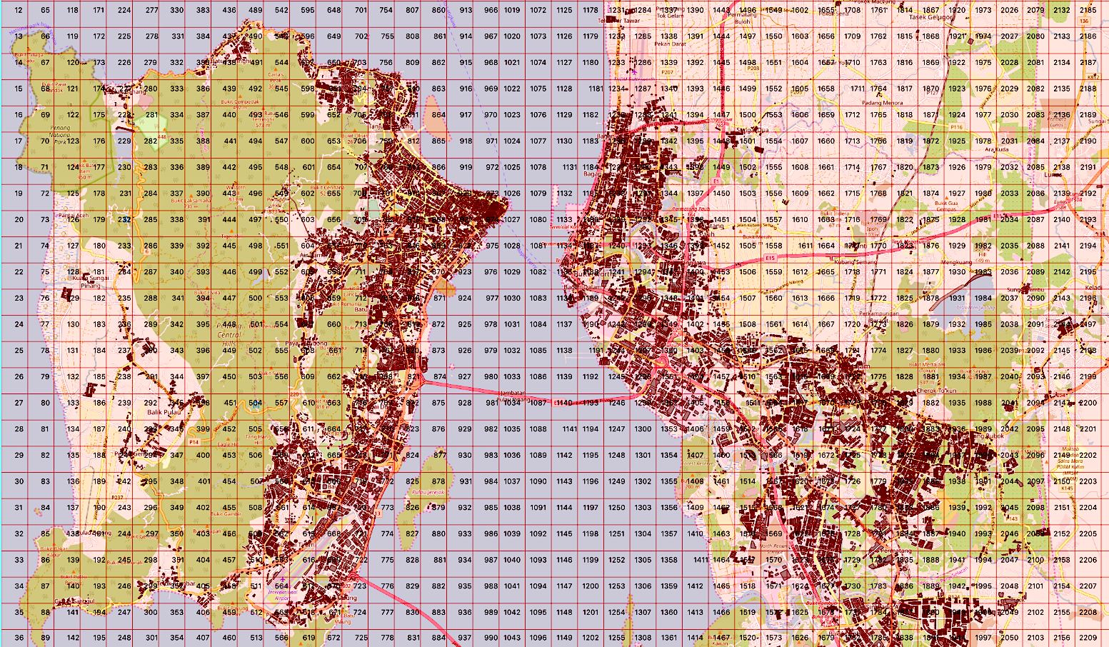
Partial view of the grid layer

In order to allocate the buildings and compute the gridwise population, we can export the boundaries information of the grids to a text file and a shape file from QGIS. The 4 boundaries of the grids are yielded in the left, top, right, and bottom columns, which follows EPSG:3857, a Spherical Mercator projection coordinate system popularized by web services such as Google and OSM. It will be converted to the normal latitude, longitude in the next step. The district column is added manually to label the parent district of the grids.

Allocation of buildings to grids

At this step, we are going to allocate the residential buildings to the grids, according to the buildings’ centric geocode and the boundaries of the grids. The coordinate systems of buildings and grids are synchronised before the allocation takes place.

import pyproj


def convert_utm_coords(coords, inProj, outProj):
    lng, lat = pyproj.transform(inProj, outProj, coords[0], coords[1])
    return pd.Series([lng, lat])


def assign_grid(coords, grid_dict):
    for grid_id, boundaries in grid_dict.items():
        if coords[0] > boundaries["left_lng"] and \
           coords[0] < boundaries["right_lng"] and \
           coords[1] > boundaries["bottom_lat"] and \
           coords[1] < boundaries["top_lat"]:
            return str(grid_id)
    return None


# Convert UTM coordinate system to latitude, longitude
inProj = pyproj.Proj(init='epsg:3857')
outProj = pyproj.Proj(init='epsg:4326')
grid_df[["left_lng", "top_lat"]] = grid_df.apply(
    lambda row: convert_utm_coords(row[["left", "top"]], inProj, outProj), axis=1
)
grid_df[["right_lng", "bottom_lat"]] = grid_df.apply(
    lambda row: convert_utm_coords(row[["right", "bottom"]], inProj, outProj), axis=1
)
grid_df["center_lng"] = (grid_df["left_lng"] + grid_df["right_lng"]) / 2
grid_df["center_lat"] = (grid_df["top_lat"] + grid_df["bottom_lat"]) / 2
grid_geocode_df = grid_df[["center_lng", "center_lat"]]

# Allocate buildings to grids
grid_dict = grid_df.to_dict("index")
buildings_df = pd.read_csv('data/penang_residential_buildings.csv')
buildings_df["grid"] = buildings_df.apply(
    lambda row: assign_grid(row[["center_lng", "center_lat"]], grid_dict), axis=1
)

buildings_df = buildings_df.set_index("id")
buildings_df.head()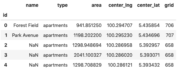

Dataframe of buildings with allocated grid

Distribution of district population into grids

This is the final step of the simulation. We are going to compute the total floor area for each grid, and allocate the district population into grids based on the gridwise total floor area.

The floor area needs to be computed separately for apartments and bungalows since they will be applied with different population densities.

buildings_df[["area", "area_bungalow"]] = buildings_df.apply(
    lambda row: check_bungalow(row["type"], row["area"]), axis=1
)

area_df = buildings_df.groupby(['grid'])['area', 'area_bungalow'].agg('sum')
area_df = pd.merge(area_df, grid_df, left_index=True, right_index=True)
area_df = area_df.drop([
    "left", "right", "top", "bottom",
    "left_lng", "top_lat", "right_lng", "bottom_lat",
    "center_lng", "center_lat"
], axis=1)

area_df = area_df.reset_index()
area_df.head()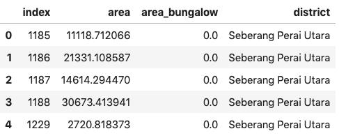

Dataframe of buildings with allocated grid

Then we can aggregate the floor area by district and estimate the population density for different districts. A uniform population density of 5 ppl / 100 m² is assumed for the bungalows.

district_df = area_df.groupby(["district"])['area', 'area_bungalow'].agg('sum')

 # Statistics obtained from Penang Institute
district_df["total_population"] = [231100, 193700, 428200, 336300, 577900]

# Assume uniform population density for bungalows: 5 ppl / 100 square meter
district_df["bungalow_population"] = district_df["total_population"] / 100 * 5
district_df["apartment_population"] = district_df["total_population"] - district_df["bungalow_population"]

district_df = district_df.reset_index()
district_df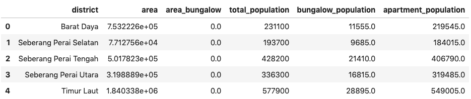

Dataframe of population for different districts

Now let’s compute the grid population based on the grid floor area, and we are done!

population_df = pd.merge(
    area_df, district_df[["district", "area", "apartment_population"]], on='district'
)
population_df = population_df.rename(columns={
    "index": "grid_id",
    "area_x": "area",
    "area_bungalow_x": "area_bungalow",
    "area_y": "area_apartment_district",
    "apartment_population": "apartment_population_district"
})
population_df["population"] = (
    population_df["apartment_population_district"] / population_df["area_apartment_district"] * population_df["area"] + \
    population_df["area_bungalow"] / 100 * 5
)
population_df["grid_id"] = population_df["grid_id"].apply(
    lambda grid_id: int(grid_id)
)

population_df.head()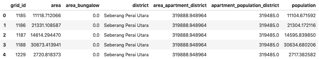

Dataframe of grid population

We can export the grid population to a shape file and generate a heatmap of population distribution on QGIS.

# Load the grids shape file exported from QGIS
sf = shp.Reader('data/penang_grid_EPSG3857_WGS84.shp')
shp_df = read_shapefile(sf)

# Append gridwise population to the grids shape
population_shp_df = pd.merge(shp_df, population_df[["grid_id", "population"]],
                             left_on='id', right_on='grid_id', how='outer')
population_shp_df["population"].fillna(0, inplace=True)
population_shp_df = population_shp_df.drop(["grid_id", "coords"], axis=1)

# Export grid population to text file
population_shp_df.to_csv('data/penang_grid_population.csv', index=False)

# Export a shape file with grid population
gdf = gpd.read_file('data/penang_grid_EPSG3857_WGS84.shp')
gdf = gdf.to_crs({'init': 'epsg:3857'})
gdf["population"] = population_shp_df["population"]
gdf.to_file('data/penang_grid_population.shp')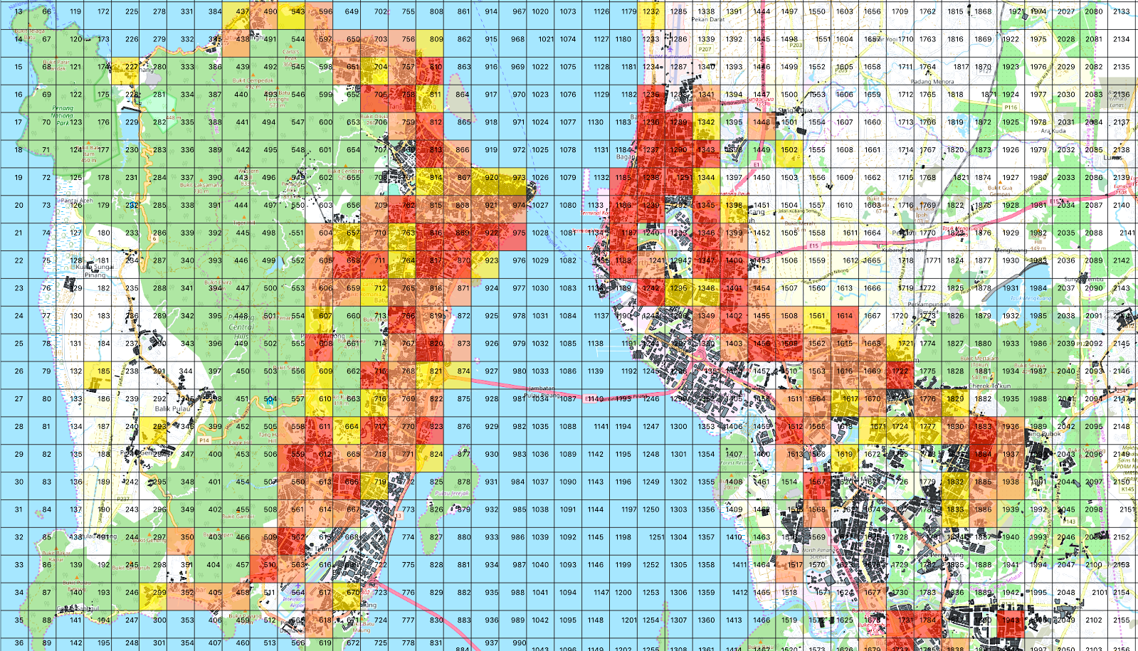

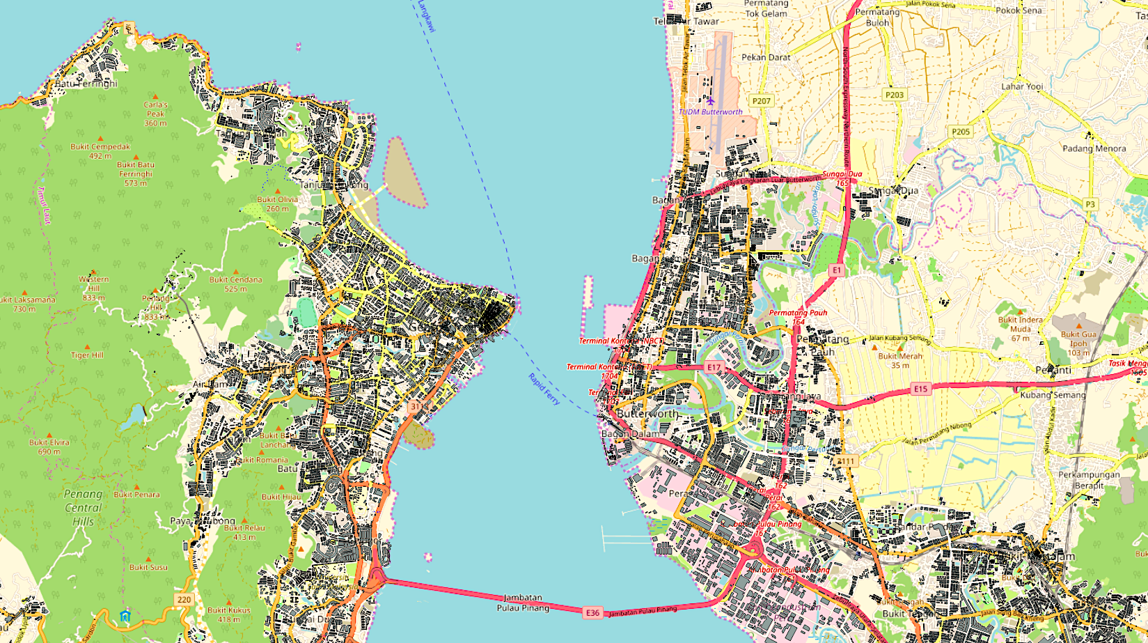
Partial view of population distribution across Penang city

In the graph, the grid population increases along with the colour temperature (from no colour, yellow, orange, to red). It can be observed that the population of Penang is concentrated mainly along the Penang Strait, forming an X shape.

The End

• We have gone through a novel approach for simulating the population distribution of a city. The solution is developed using open-source tools and OSM dataset.
• Some error is expected due to the assumption of uniform residential density. In addition, the OSM data itself might not be 100% correct and up to date.

Thanks for the read. The codebase is available on GitHub.